


Machine learning workshop Report
Real estate price prediction - 2022
CHOUKRI Réda (ISSD & IRIV ID) LOEHRER Léo (ISSD),ELMAHI Aymane (SDIA) BERTRAND Simon (ISSD & IRIV ID)
The problem of housing price prediction is a significant challenge that has been the focus of research and attention in the real estate and economic fields. Housing prices play a critical role in the economy and have a significant impact on a variety of industries, including banking, real estate, and construction. Accurately predicting housing prices is essential for informed decision-making, whether it be for buying, selling, or investing in real estate.
Traditionally, housing price predictions have been based on human expertise and experience, which has its limitations. This approach is time-consuming and may not always lead to accurate results, especially in rapidly changing and complex markets. With the advancement of technology and the availability of vast amounts of data, machine learning has emerged as a powerful tool for addressing this challenge. Machine learning algorithms can process large amounts of data, identify patterns, and make predictions with a high degree of accuracy, making it a promising approach for housing price prediction.
This problem is especially relevant in today's fast-paced and data-driven world, where the ability to make accurate and timely predictions is critical. In this context, the development of a machine learning model for housing price prediction has the potential to provide valuable insights and support informed decision-making in the real estate industry.
In this challenge, our objective is to develop an effective machine learning model for housing price prediction. The model will be trained on a provided training dataset and its performance will be evaluated based on its ability to make accurate predictions. To achieve this goal, we will explore different machine learning approaches and algorithms, including regression and decision tree methods, to develop our final model.
The results of this challenge will have significant implications for the real estate industry, providing a valuable tool for making informed decisions about buying, selling, or investing in property. As data scientists, we are excited to tackle this challenge and to see how our model performs. This project will allow us to apply our skills and knowledge to a real-world problem and make a meaningful contribution to the field of housing price prediction.
The main difficulty of this subject is to integrate the images data to observe if the presence of the latter can increase the accuracy of the model. We understood that, without the images data, the regression results of the tabular data was not good enough and we concluded that it was useless to train the model only on the tabular data. As we can have up to 1 to 6 images per observation and that we have different images width and height, we called this aspect a “dynamic” dimension because the total number of pixels can be different from one observation to another. The problem with the dynamic dimension is that it makes the model architecture more difficult to create. The original subject proposed a strategy to get to the end of this problem, by just replacing the images data by three new features that contain respectively the mean quantity rate of red, green and blue pixels for each multiple image observation. This would transform the dynamic dimension to a static one, but we did not understand how a mean quantity rate of pixel colors can have an influence on the price target.Through a simple thought exercise, we imagined giving a real estate expert these different rates so that he could give us a better estimate of the price, which seemed unrealistic. The main problem with this technique was maybe a too drastic reduction in the dimension of the image data. We decided in consequence of this thought process that we should reduce the image's data dimension to a much larger one. This should filter useless data but also extract interesting features from the images. The main ideas of our subject were about the preprocessing step, and more precisely, the transformation of the images data to an efficient concentration of information, tabular data that we could concatenate to the other tabular data. We wanted also to transform each feature of the basic tabular data to a score feature which uses an a priori knowledge or not, in order to estimate the price of the observation.
1. Visualization
The dataset consists of 27 features, including the price of the estate and photos of the estate, summarized in the following table.
| Features | Categorical or Continuous | Description |
|---|---|---|
| Property type | Categorical | Type of the estate (22 differents type) |
| Latitude | Continuous | Latitude position |
| Longitude | Continuous | Longitude position |
| City | Categorical | Name of the city where the estate is sold |
| Postal code | Categorical | Postal code of the city |
| Size | Continuous | Living space |
| Floor | Categorical | Stage of the estate |
| Land size | Continuous | Outside space |
| Energy performance value | Continuous | Estimated energy consumption (kWh/m²/year) |
| Energy performance category | Categorical | French energy rating |
| Greenhouse gas emission value | Continuous | Green gas emission estimated (kg eq CO2/m²/year) |
|---|---|---|
| Greenhouse gas emission category | Categorical | French energy rating |
| Exposition | Continuous | Estate orientation |
| Number of rooms | Categorical | Number of rooms |
| Number of bathrooms | Categorical | Number of bathrooms |
| Number of bedrooms | Categorical | Numbers of bedrooms |
| Has a parking place | Categorical (Boolean) | Parking place (Yes/No) |
| Has boxes | Categorical (Boolean) | Boxes (Yes/No) |
| Numbers of photos | Categorical | Numbers of photos of the estate |
| Has a balcony | Categorical (Boolean) | Balcony (Yes/No) |
| Has a terrace | Categorical (Boolean) | Terrace (Yes/No) |
| Has a cellar | Categorical (Boolean) | Cellar(Yes/No) |
|---|---|---|
| Has a garage | Categorical (Boolean) | Garage (Yes/No) |
| Has air conditioning | Categorical (Boolean) | Air conditioning(Yes/No) |
| Last Floor | Categorical (Boolean) | Last Level(Yes/No) |
| Upper Floor | Categorical (Boolean) | Ground level(Yes/No) |
| Price | Continuous | Price of the estate |
| The features can be grouped into smaller sets to simplify visualization and reduce the number of dimensions. However, not all features have equal impact on the estate's price. Understanding the type of estate being sold is critical, while exposure is not a key factor in the evaluation. Thus, only the essential features for the estimation will be visualized. |
This feature ‘property type’ is considered a crucial aspect for obtaining an accurate estimation.

The histogram above depicts the count of each property type in the dataset. We can see that apartments and houses are the most common types, accounting for 84% of the data. The remaining 10% is split between miscellaneous and field types, while the remaining 6% is split among 18 other types. The dataset includes a total of 22 different types. Given the significance of this feature, we decided to investigate the missing values in the dataset by creating a heatmap of the missing value proportions for each property type and other features.

The features not displayed on the heatmap have no missing values, whereas a value of 1 on the heatmap indicates 100% missing values. The heatmap serves as a useful tool in directing the pre-processing steps. One key observation is the number of property types with 100% missing values in the "floor" feature, which is expected since most estates except apartments, rooms, and duplexes are on the ground level. As such, these missing values will be filled with 0. Another observation is the similar proportion of missing values in the four energy consumption related features, which can be grouped together. However, since houses and apartments make up the majority of the dataset and have missing value proportions of 0.4 and 0.5 respectively, these features will not be used in the price prediction. Only 4 estates of the type "lodge" or "hotel" are sold, so no special pre-processing will be performed for this type of estate.
2. Preprocessing on the images
Image Captioning is the task of generating a textual description for an image, which requires understanding the visual contents of the image and being able to translate that information into words. This task has a wide range of applications, such as assisting visually impaired individuals, improving image retrieval systems, and providing additional information for multimedia content. In our case, we used it to transform the images into tabular data as explained above.
For this we tried to use pre-trained models published on paperswithcode.com, first we used the MPLUG model, it is an innovative cross-modal learning framework that aims to effectively and efficiently learn vision-language relationships by combining the power of visual and textual features through cross-modal skip-connections, MPLUG uses a deep learning technique to generate image descriptions, which involves training multiple layers of neurons. Our computers do not have enough processing power to train these layers efficiently.
YOLOv7 was also an option we considered at first and spent a lot of time on. YOLO has a reputation for being fast and accurate, and we thought that it would be well-suited for the task of identifying objects and their attributes within images
However, as I delved deeper into the specifics of YOLO and its requirements, I quickly realized that the algorithm would need to be trained in order to achieve the level of accuracy and performance we were seeking.
On the same site we found an alternative, LAVIS Model, which is an architecture for language-image pre-training that was introduced in the paper "Bootstrapping Language-Image Pre-training with Frozen Image Encoders and Large Language Models." The model is based on the idea of combining the strengths of large language models (such as GPT) and image encoders (such as ResNet) to improve the performance of vision-language tasks. The architecture consists of two main components: a frozen image encoder and a large language model. The image encoder is pre-trained on large-scale image classification tasks, while the language model is fine-tuned on vision-language tasks using the representations generated by the image encoder. The model is trained in a multi-stage process, where the image encoder is first trained, followed by the fine-tuning of the language model. This approach allows the model to leverage the knowledge gained from the pre-training of the image encoder and the fine-tuning of the language model to improve the performance of vision-language tasks.
The LAVIS model, or BLIP-2, uses two datasets: Base_COCO and Large_COCO. Base_COCO is a smaller version of the Common Objects in Context (COCO) dataset, which contains 330,000 images and 2.5 million object annotations. The Large_COCO dataset is a larger version of COCO, which contains 2.5 million images and 33 million object annotations. Both datasets are widely used for computer vision and natural language processing tasks, and provide a diverse set of images with complex annotations, including object instances, captions, and keypoints. The Base_COCO dataset is used as a pre-training dataset, while the Large_COCO dataset is used for fine-tuning the model on specific tasks. In our case we used the Base_COCO dataset..
As soon as we installed the model, we tried to create a data frame which contains two columns "id_annonce" and "captions", the captions column contains a list of captions each corresponding to an image, we have more than 37k rows, and on average each row contains 5 images, the time needed to extract the caption from the image is 2s, so we were on 82h to transform the whole dataset, for that we considered several solutions such as :
PySpark is a distributed data processing library using Apache Spark. Spark is a highly parallel data processing framework that allows complex tasks to be performed on large datasets in parallel across multiple nodes in a cluster. Using PySpark, data can be distributed across multiple nodes for faster and more efficient processing.
This solution was not the most adapted to our case, we were able to optimize the execution time, we went from 82h to 63h, but it was not enough because we were limited by the number of nodes, given the modest performances of our computers, we could not launch on a large number of nodes.
Asyncio is a Python module for asynchronous programming that provides efficient handling of non-blocking I/O. It allows applications to not get stuck waiting for slow operations and to run multiple tasks in parallel, which can optimize execution time. It uses a "task" approach to organize the different elements of an application and have them run in parallel rather than sequentially, which can significantly reduce the overall execution time.
we divided our dataset to batches with 50 lines per one, and with Asyncio we can apply the transformation on 50 lines in parallel, which will reduce 50 times the execution time, but the functions used in the pre-training model we used are blocking, so we could not preserve the asynchronous character of Asyncio.
To achieve the preprocessing step correctly, we used the above-mentioned AI model to transform our images data but we didn’t have the computing power even with the PySpark and Asyncio methods. So we asked our professors to have SSH access to a GPU station with a GTX 3080 that is compatible with CUDA to faster generate captions using a multithreading technique. The script we ran on the machine was executing a batch of 8 threads at once where each thread was generating captions for 50 observations (a mean of 150 images). We were running 400 observations at once using the thread method which allowed us to execute the script in 13 hours to generate the captions for the 300K photos. In comparison with our machines, using the best of them, we would have taken 63 hours to generate these captions. We could have divided these >63 hours by the number of machines we have, but this was too much handicraft.
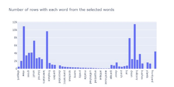
Upon execution of the script on the GPU station, the captions were gathered and subjected to filtering processes. A dictionary was generated to encompass all relevant words and their respective frequency. The resulting dataframe is as follows:

Subsequently, the repetition of non-informative words, commonly referred to as stop words ("a", "an", "and", "are", "as", "at", "be", "by", "for", etc.), were removed to obtain a final dictionary illustrated as follows:

Following the removal of stop words, we engaged in a deliberation process to determine which words were of sufficient relevance to have an impact on building prices. Multiple combinations were explored and after thorough analysis, it was determined that adjectives such as "elegant", "unique", and "spacious" held significant importance. The dataframe was then updated to include these key terms as columns, transforming the images into structured data. The words we decided to keep are the following :
["elegant", "pool", "view", "big", "grass","tub","small","hallway","blurred","patio","lawn", "stairs", "tree", "fireplace", "artistic", "garden","modern","bright", "decorated", "fashioned", "panoramic", "high", "spacious","beautiful", "sunny", "colors","pretty", "chandelier", "marble", "messy","unfinished", "shining", "organized", "huge", "antique","renovated", "warehouse", "rooftop","garage","swimming", "decor","loft","porch","umbrella", "bar","wooden","clean", "empty","balcony","tile", "bushes","nice","good", "plants","backyard","frontyard","yard"]
3. Preprocessing on tabular data
The chosen features for estimation include:
- Property type
- Localization (City, Latitude, Longitude)
- Size of the estate
- Floor
- Land size of the estate
- Rooms (number of rooms, bedrooms and bathrooms)
- Boolean (Parking place, boxes, balcony, terrace, cellar, garage, air conditioning, last floor, upper floor)
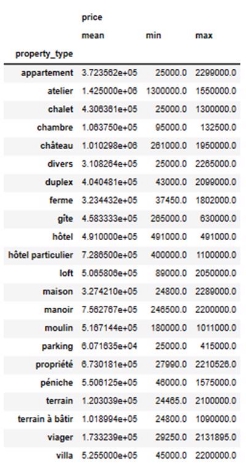
Concerning the property type, the categorical data will be converted to numerical data by using a Score function. The 22 property types will be reduced to 6 categories based on the mean of each type and physical similarities of the estate.
A table with the mean, minimum, and maximum of each property type is available in the annex (1). The score function will compute the mean of each category and normalize it between 0 and 1, with Category 1 being equal to 1 and Category 6 being equal to 0.
Resume Table
| Property type | Category | Score |
|---|---|---|
| Château, atelier, hôtel particulier, manoir, péniche, villa, moulin, loft, propriété | 1 | 1 |
| Duplex, chambre, appartement | 2 | 0.54 |
| Chalet, ferme, gîte, viager, maison | 3 | 0.49 |
| Hôtel, divers | 4 | 0.37 |
| Terrain, terrain à bâtir | 5 | 0.06 |
| Parking | 6 | 0 |
| Localization Information: City, Latitude, Longitude, and Postal code provide crucial spatial details, particularly when paired with the property type. This is because the cost per square meter can differ greatly between cities. |
The main challenge with this data is the vast number of cities represented (over 8,000). These cities are categorical data that are unrelated to other features in the dataset. To address this issue, we will implement a regression model to generate a score based on the city, latitude, and longitude features.
Initially, a CSV file will be created with the names of 50 major cities throughout France. Each city will be listed with its latitude and longitude, as well as the cost per square meter.

Ten first cities in the dataframe
For each of the 50 cities, a Gaussian is placed with a mean of the city's latitude and longitude and a standard deviation of 0.1. The probability density for each city in the dataset is then calculated relative to the reference cities. The resulting probability densities are normalized by summing them, and then multiplied by the respective city's price per square meter. This provides a price per square meter for each city, based on its position relative to the reference cities.

Let i denote the i-th city among the top 50 major cities. The density probability for each city is represented by Pdf(i), with mean (latitude(i), longitude(i)) and variance var(x)² = var(y)² = 0.1, as well as covariance cov(x,y) = 0. The price per square meter for each city is represented by Price(i).
The correlation coefficient between the price and the score of a city is 0.4. Based on this, a hierarchy has been created for the categorical data of cities.
The size of the property is also a significant factor in determining its price. Therefore, this feature will be pre-processed with the "land size" feature, taking into account different property types. For example, apartments typically do not have a garden, so the "land size" value will be 0. However, the "land size" feature is missing in the dataset. For fields, the "size" and "land size" values are equal, avoiding double counting and potential biases in the model. Before proceeding, the data will be visualized.

For apartments and houses, it can be observed that larger properties tend to be more expensive. Thus, this hierarchy will be maintained, and the "size" and "land size" features will be pre-processed using the following rules:
- If the property type is "terrain" or "terrain à bâtir", the "size" will be set to 0, and the field size will be stored in the "land size" feature.
- If "size" is missing and "land size" is not missing, "size" will be set to "land size" and "land size" will be set to 0.
- If "size" is missing, it will be set to 0.
- If "land size" is missing, it will be set to 0.
- In all other cases, the original values will be maintained.
The decision to set missing values to 0 was made to avoid introducing a large bias, which would reduce the accuracy of the model during the training phase.
The floor feature will only be useful for properties that are not at ground level, such as apartments, duplexes, and rooms. We will visualize the data to better understand its usefulness.

From the data visualization, it is evident that the higher the level, the higher the price. Our prior knowledge suggests that the price increase will be greater when moving from level 3 to level 4, compared to when moving from level 12 to level 13. To incorporate this knowledge, missing values for the "floor" feature will be replaced by 0, as they correspond to ground level. The score function for the "floor" feature will also compute the logarithm of the floor, thus increasing the difference between small consecutive values and reducing the difference between larger consecutive values.
The features "number of rooms", "bedrooms", and "bathrooms" convey similar information, so we will combine them into one feature by using just "number of rooms". Before doing so, let's visualize the data.

The graph clearly shows that the higher the number of rooms, the higher the price. The correlation coefficient between price and number of rooms is 0.44 and the proportion of missing values in the entire dataset for this feature is less than 1%. Thus, we will retain the number of rooms as is and replace missing values with 0.
Since this data contains no missing values, it will be beneficial to include as a value that can add a positive or negative impact to the estate, such as an upper level. Thus, these data will be kept as is.
1. Definition of the regression algorithms used
Our goal is to perform regression on the data using the scikit-learn library, which provides various regression algorithms and evaluation/validation metrics, normalization capabilities. We will be evaluating the performance of four different algorithms and selecting the best one among them. The algorithms tested are:
MLP Regressor : is a type of neural network algorithm that is used for regression tasks. It uses multiple layers of artificial neurons to learn the relationships between the input features and the target values.
Decision Tree Regressor : is a tree-based algorithm that splits the input data into smaller groups based on the values of the features. The prediction is made by considering the average of the target values in each group.
SVM Regressor : is a type of regression algorithm in which a Support Vector Machine (SVM) model is used to predict a continuous target variable. It uses the SVM algorithm to fit a line or hyperplane to the input data in a high-dimensional feature space and find the best boundary that separates the data into the respective classes.
Lasso Regressor : is a type of linear regression algorithm that adds a regularization term to the loss function in order to prevent overfitting. The regularization term is based on the L1 norm, which encourages the model to have sparse coefficients, i.e., it only includes the most important features in the prediction.
2. Appropriate hyperparameters for each algorithm
The best hyperparameters for each algorithm were found by using RandomizedSearchCV, which is a method that randomly searches the hyperparameter space for the best combination of hyperparameters.
For the MLPRegressor, the best hyperparameters were found to be: activation function as "relu", alpha value of 0.0001, hidden layer sizes of (50, 100, 50), a constant learning rate, and a maximum number of iterations of 100.
For the DecisionTreeRegressor, the best hyperparameters were found to be: a criterion of "mse", a maximum depth of 20, a minimum number of samples per leaf of 4, a minimum number of samples required to split an internal node of 10, and a splitter of "best".
For the SVMRegressor, the best hyperparameters were found to be: a maximum number of iterations of 500, a kernel of "linear", a gamma value of 10.0, and a C value of 1.0
For the LassoRegressor, the best hyperparameters were found to be: alpha value of 100.0, a fit_intercept of True, a normalization of False, a precompute of True, and a selection of "cyclic".
3. Evaluation
Having determined the optimal hyper-parameters for each regression algorithm, we can now compare their performance. To do so, we performed a cross validation and analyzed the learning curves for each algorithm.
- MLPRegressor:
The cross-validation scores range from 0.30 to 0.41, with an average of 0.36. This shows that the MLPRegressor is not capable of producing fairly accurate predictions, but it is possible to further improve the performance.
In the learning curve below, we can see that the more data we have the more the training loss and CV loss decrease, so maybe the model needs more data to train well, otherwise the Learning Curves in this case are Showing a Good Fit

Fig. MLPRegressor learning curve
- DecisionTreeRegressor
Has cross-validation scores between 0.44 and 0.49, with an average of 0.4, compared to the MLPRegressor the DecisionTreeRegressor shows a good level of performance.
In the learning curve below, we can see that the model learned well on the training data, as well as the decrease of cross validation loss with the increase of the training data size, so if we had more data, the model could reach its maximum performance!

Fig. DecisionTreeRegressor learning curve
- SVMRegressor
SVM has negative cross-validation scores, with an average of -1.07. This suggests that SVR is not the best choice for the current data.
If the data is not linear, SVM may not be the best choice as it is more suitable for linear pattern recognition.
- LassoRegressor
Finally, for Lasso, the cross-validation scores range from 0.30 to 0.38, with an average of 0.34. While this is not as high as MLPRegressor or DecisionTreeRegressor, Lasso shows an acceptable level of performance for regression.
On the learning curve below, the shaded area represents the confidence interval of the training error. It shows the variability of the training errors for each training set size. More precisely, it shows the difference between the mean of the training error and its upper and lower standard deviations. So we can see that we have a large dispersion of training errors

In conclusion, based on the results of the cross-validation and the learning curve analysis, the DecisiontreeRegressor seems to be the best regression algorithm for the current data, closely followed by the MLPRegressor.
a. Metrics
The model chosen to make predictions on the full dataset is a DecisionTreeRegressor with a maximum depth of 20, a minimum of 4 samples per leaf and a minimum of 10 samples to split.
To evaluate the performance of our model we used the Mean Squared Error (MSE), R-Squared and Root Mean Squared Error (RMSE) metrics.
- MSE measures the mean squared error between the actual and predicted targets.
- RMSE measures the mean squared error, expressed in units of the target
- R-Squared measures the correlation between actual and predicted targets.
Test on the training data
We evaluated the model on the training data we found an RMSE of about 133000 euros, which is not negligible, we also found an R-Squared of 81%, which shows that the model has been well trained on the training data, and from the graph below, we can visualize the correlation of ground truth and the prediction, the graphical results are well consistent with the theoretical results.

Fig. The prediction versus the actual target (Train Data)
Test on the test data
The results show that the performance of the model on the test data is poor, with an R-squared coefficient of 0.49, which indicates that just 49% of the variation in house prices can be explained by the characteristics of the property. The RMSE is around 225,000 euros, which gives an idea of the average error between the predicted and actual values.
In the graph below, we can see that the predicted data and the actual data are not well correlated, which is consistent with what we mentioned earlier.

Fig. The prediction versus the actual target (Train Data)
As a conclusion to the original problem, we were unable to derive any conclusive information from the images that could improve the tabular model. As the evaluation metrics were not excellent, we could have transformed the regression problem into a classification problem by grouping the prices in successive bands of 25k€ or 50k€. In order not to have to deal with the dynamic dimension of the images, we would then have had to find another dimension reduction technique during preprocessing that would have been able to extract more knowledge from the images, without filtering it too much, or not enough.
According to the found metric values and the graphical analysis, we can conclude that our model is not performing well when faced with new data. There may be several reasons for this, including our strategy for exploiting the images. We have tried to carefully choose the keywords that appear in order to avoid biasing the model, especially since we have no control over what the Lavis model returns. It's also possible that none of the selected words appear in the captions of the images our model was tested on. To enhance the model's performance, we could have considered including synonyms of our words in the same column. This would allow the model to recognize that words such as "elegant" and "pretty" have a similar effect.
What we could also consider doing in the future is to train our image captioning model ourselves on well-chosen and well-labeled data in order to have captions that describe what is in the images in a precise manner.
Annex
(1)